Getting Started
- Obtaining NIMH MonkeyLogic
- Software Installation
- Using a MATLAB app installer
- Using a ZIP file
- Installing additional libraries
- A tip for future upgrades
- Starting NIMH MonkeyLogic
- Eye #1: Mouse cursor
- Eye #2: 'I', 'K', 'J', 'L'
- Joystick #1: Arrow keys (↑, ↓, ←, →)
- Joystick #2: 'W', 'S', 'A', 'D'
- Touch: Mouse left click & right click
- Buttons: '1', '2', '3', '4', '5', '6', '7', '8', '9', '0'
- File Formats Supported by NIMH MonkeyLogic
- Aligning Timestamps and Analog Data
- Migrating from the Original MonkeyLogic
- Configuration file
- TrialRecord
- Movie frame rate
- Reaction time
NIMH ML is downloadable from https://monkeylogic.nimh.nih.gov/download.html.
Either a MATLAB app installer or a ZIP file can be used for installation.
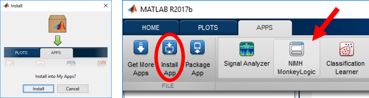
Double-click the downloaded *.mltbx file. It will open MATLAB and insatall NIMH ML. Upon completion, NIMH ML will be added to the MATLAB menu as shown below. If this process fails for any reason, manually open MATLAB and install the package by clicking the [Install App] menu.
Decompress the zip file to a directory and add that directory to the MATLAB path. The subdirectories can be added, but that step is not necessary.
Windows N needs the Media Feature Pack to run NIMH ML. It is an optional feature of Windows N that is freely available.
If you have a parallel port, NIMH ML will ask to install InpOutx64, an open source parallel port driver. To install it, run inpoutx64_installer.exe in the daqtoolbox directory of the NIMH ML installation path. The admin privilege is required. The installation occurs instantly and there is no wizard window showing up.
Old versions may require Visual C++ Redistributable or DirectX End-User Runtime. Please follow the instructions displayed on the MATLAB command window on startup.
Keep your task files separately outside the NIMH ML installation directory. NIMH ML does not store anything in its main directory, so deleting the main directory is safe if your files are stored elsewhere.
Click the [NIMH MonkeyLogic] icon on the MATLAB APPS menu (if NIMH ML was installed with the MATLAB app installer) or type "monkeylogic" on the MATLAB command window (if it was installed with the ZIP file).
NIMH ML comes with many example tasks (see the "task" directory in the NIMH ML installation path). To start a task, choose a conditions file by clicking the [Load a conditions file] button on the ML GUI (left figure below) and then hit the [Run] button.

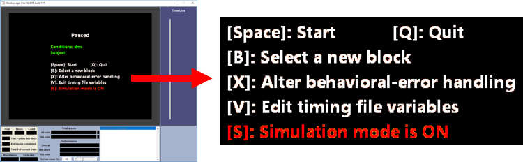
It is possible to run a task without a DAQ board or any input device, by activating the simulation mode in the pause menu. In the simulation mode, most input signals are replaced with mouse and key inputs shown here.
For more information about how to run tasks, see "Running a Task".
NIMH ML supports its own data file format, called BHV2 (*.bhv2), as well as HDF5 (*.h5) and MAT (*.mat). BHV2 is a private format that is based on a simple recursive algorithm (see "BHV2 Binary Structure" in the appendix). It provides decent read and write performance and is recommended for most users. HDF5 is supported by many commercial and non-commercial software platforms, including Java, MATLAB, Scilab, Octave, Mathematica, IDL, Python, R and Julia, but its read performance in MATLAB is a bit disappointing. MAT is MATLAB’s native data format. NIMH ML uses the default MAT-file format that is set in the MATLAB Preferences. The MAT file format has a weakness in that it gets slower as more and more variables are stored, even though file compression is disabled.
BHVZ is BHV2 with zip compression. It is slower than BHV2 but saves considerable disk space.
The mlread function provides a unified read interface for all the formats. It returns trial-by-trial data in a 1-by-n struct array.
data = mlread;
data = mlread(filename);
[data, MLConfig, TrialRecord, filename] = mlread(__);
The mlconcatenate function combines trial-by-trial analog data into one large seamless matrix and adjusts all timestamps accordingly, as if the data were recorded in one single trial. This function is especially useful for reading data files in which signals were continuously recorded through inter-trial intervals.
data = mlconcatenate;
data = mlconcatenate(filename);
[data, MLConfig, TrialRecord, filename] = mlconcatenate(__);
Some recorded signals, such as High Frequency, Voice or Webcam, have a large size and loading them all at once may cause an out-of-memory error. Those signals are stored as separate variables and not processed by mlread nor mlconcatenate. To read those data, use the mlreadsignal function.
signal = mlreadsignal(signal_type); % 'high1', 'voice', 'cam2', etc.
signal = mlreadsignal(signal_type, trial_num);
signal = mlreadsignal(signal_type, trial_num, filename);
[video, timestamp] = mlreadsignal('webcam1' ,__); % 'webcam' + cam#
Saved file-source stimuli in the data file can be retrieved with the mlexportstim function.
mlexportstim;
mlexportstim(destination_path);
mlexportstim(destination_path, datafile);
In NIMH ML, a trial starts at Time 0 and so does data acquisition. Therefore, matrix indices to address analog data for a particular period can be calculated from the time of the period. For example, to get eye traces for an epoch marked by Eventcodes 10 and 20, write a script as below.
data = mlread;  % read a data file
trial_no = 1;
code = data(trial_no).BehavioralCodes.CodeNumbers;
time = data(trial_no).BehavioralCodes.CodeTimes;
eye = data(trial_no).AnalogData.Eye;

start_time = time(find(10==code,1));  % time is in milliseconds.
end_time = time(find(20==code,1));

start_index = round(start_time) + 1;  % data is sampled at 1 kHz.
end_index = round(end_time) + 1;

segment = eye(start_index:end_index,:);
NIMH ML uses Eventcodes 9 (Start trial) and 18 (End trial) to mark the boundaries of a trial in the neural data stream. Note that the timestamps of those codes are just the times that the codes were sent to the neural recording system and not the actual start time and end time of a trial, despite the code labels. To get precise trial intervals, use the AbsoluteTrialStartTime field, which indicates the time elapsed from the beginning of Trial 1 (in milliseconds).
NIMH ML is designed to run the scripts written for the original ML seamlessly. However, there are a couple of things that you should keep in mind when migrating from the original ML to NIMH ML.
The configuration file of the original ML (*_cfg.mat) is not compatible with that of NIMH ML (*_cfg2.mat), so creating a new configuration file is necessary after installing NIMH ML.
In the original ML, custom fields could be added to TrialRecord to pass user variables around. In NIMH ML, such a trick is not allowed, because TrialRecord is a class object, not a struct. If you need custom fields, use TrialRecord.User instead.
TrialRecord.var1 = 200;       % fine in the original ML, but not in NIMH ML
TrialRecord.User.var1 = 200;  % good with NIMH ML
Note that the fields you create under TrialRecord.User are not automatically saved to the data file. You should use the bhv_variable function to keep the records of them.
The original ML presents movies frame by frame, so their duration varies depending on the refresh rate of the screen. NIMH ML plays movies at a constant speed, regardless of the refresh rate. See this to play movies in the same way as the original ML does in NIMH ML.
At the end of each trial, the value assigned to a variable, 'rt', is used to update the default reaction time graph in the control screen. It is also stored in TrialRecord.ReactionTimes and the data file for online and offline reference, respectively.
In the original ML, the reaction time that eyejoytrack() returns is calculated from the beginning of eyejoytrack(). Since stimuli are presented by toggleobject() before eyejoytrack() starts, this produces a number slightly shorter than the time measured from the stimulus onset, although the difference is small.
toggleobject(1);
[ontarget, rt] = eyejoytrack('acquirefix' ,1,3,1000); % rt measured from the start of eyejoytrack()
NIMH ML still supports the above method and also provides a way to calculate the reaction time from the stimulus onset.
t_flip = toggleobject(1);
[ontarget, ~, t_resp] = eyejoytrack('acquirefix' ,1,3,1000); % Only NIMH ML returns the 3rd output
rt = t_resp - t_flip;
In case you program in the style of Timing Script v2 (a.k.a. Scene Framework), you can calculate the reaction time like this:
t_flip = run_scene(scene);      % Assume that the scene includes a WaitThenHold (wth) adapter
rt = wth.AcquiredTime - t_flip; % t_flip is the time that the 1st frame of the scene was presented
or simply
rt = wth.RT;
Currently these adapters have the AcquiredTime and RT properties: WaitThenHold, FreeThenHold, MultiTarget, OnsetDetector